Page 224 - MATLAB an introduction with applications

Numerical Methods ——— 209

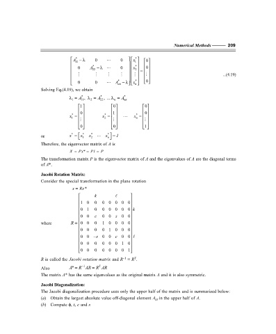
 A −λ 0 " 0  x  *  0 
*
 11   1  
*
0
 0 A −λ " 0  x  * 2  
22
 # # # #   #  = #  ...(4.19)
    
 0 0 " A −λ   x *  
0 
*
 nn   n 
Solving Eq.(4.19), we obtain
*
*
λ= A 11 , λ = A * 22 , ... λ = A nn
1
2
n
1  0  0 
  
0
1
0
*
*
*
x =  x =  " x = 
# 
1 # 2 #  n 
  
0 
1 
0 
  
*
*
or x =  x  1 * x 2 * " x  = I
n 
Therefore, the eigenvector matrix of A is
X = Px * = PI = P
The transformation matrix P is the eigenvector matrix of A and the eigenvalues of A are the diagonal terms
of A*.
Jacobi Rotation Matrix:
Consider the special transformation in the plane rotation
x = Rx *
 k A 
 1 0 0 0 00 00 
 
 01 0 0 00 00 k 
 
 00 c 0 0 s 00 
where R =  00 0 1 00 00 
 
 0 0 0 0 1 0 0 0 
 00 − s 0 0 c 00 A

 
 00 0 0 001 0
 
  00 0 0 00 01 
–1
R is called the Jacobi rotation matrix and R = R .
T
−
T
1
A
Also * = R AR = R AR
The matrix A* has the same eigenvalues as the original matrix A and it is also symmetric.
Jacobi Diagonalization:
The Jacobi diagonalization procedure uses only the upper half of the matrix and is summarized below:
(a) Obtain the largest absolute value off-diagonal element A in the upper half of A.
kA
(b) Compute φ, t, c and s