Page 228 - MATLAB an introduction with applications

Numerical Methods ——— 213

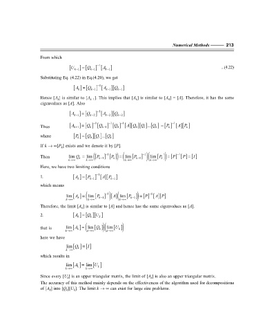
From which

−
1
=
[U k− 1 ] [Q k− 1 ] [ k− 1 ] ...(4.22)
A
Substituting Eq. (4.22) in Eq.(4.20), we get
−
1
A =
[ ] [Q k− 1 ] [ k − 1 ][Q k− 1 ]
A
k
Hence [A ] is similar to [A ]. This implies that [A ] is similar to [A ] = [A]. Therefore, it has the same
k
k
0
k–1
eigenvalues as [A]. Also
A = − 1 A ]
[ k − 1 ] [Q k − 2 ] [ k − 2 ][Q k − 2
−
−
−
−
1
1
1
1
=
=
Q
A Q
... Q
Q
A
Q
P
A P
Thus [ k+ 1 ] [ ] [Q k− 1 ] [ ] [][ ][ ] [ ] [ ] [][ ]
0
1
k
k
0
k
k
P =
... Q
Q
Q
where [ ] [ ][ ] [ ]
k
0
1
k
If k → ∞[P ] exists and we denote it by [P].
k
[ ])
[ (
−
−
−
1
1
1
=
P =
P
P
Then lim Q = lim P k− 1 ] [ ]) ( lim P 1 ] )( lim P k = [] [] [ ] I
[ k−
k
k
k→∞ k→∞ k→∞ k→∞
Here, we have two limiting conditions
−
1
A =
A P
P
1. [ ] [ k− 1 ] [][ k− 1 ]
k
which means
[ ] (
−
−
1
1
lim A = lim P 1 ] ) []( lim P 1 ]) = [] [ ][] P
A
A
P
[ k −
[ k −
k
k→∞ k→∞ k→∞
Therefore, the limit [A ] is similar to [A] and hence has the same eigenvalues as [A].
k
A =
U
Q
2. [ ] [ ][ ]
k
k
k
[ ])(
[ ])
[ ] (
that is lim A = lim Q k lim U k
k
k→∞ k→∞ k→∞
here we have
[ ] [] I
lim Q =
k
k→∞
which results in
[ ]
[ ] =
lim A k lim U k
k→∞ k→∞
Since every [U ] is an upper triangular matrix, the limit of [A ] is also an upper triangular matrix.
k
k
The accuracy of this method mainly depends on the effectiveness of the algorithm used for decompositions
of [A ] into [Q ][U ]. The limit k → ∞ can exist for large size problems.
k
k
k