Page 226 - MATLAB an introduction with applications

Numerical Methods ——— 211

4.13 STURN SEQUENCE

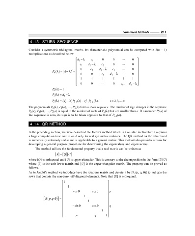
Consider a symmetric tridiagonal matrix. Its characteristic polynomial can be computed with 3(n – 1)
multiplications as described below:
 d −λ c 1 0 0 " 0 
1
 c d −λ c 0 " 0 
 1 2 2 
 0 c d −λ c " 0 
P n () λ= A − λ =  2 3 3 
I
 0 0 c 3 d −λ " 0 
4
 # # # # # # 
 
  0 0 " 0 c n− 1 d −λ 
n
λ=
P 0 () 1
P 1 ()λ= d − λ
1
2
P λ i )P i− 1 ( ) c P 2 ( ), i = 2,3,...,n
( ) = (d − λ
λ
λ −
i−
1 i−
i
The polynomials P (λ), P (λ), …, P (λ) form a sturn sequence. The number of sign changes in the sequence
n
1
0
P (a), P (a), …, P (a) is equal to the number of roots of P (λ) that are smaller than a. If a member P (a) of
1
n
0
i
n
the sequence is zero, its sign is to be taken opposite to that of P (a).
i–1
4.14 QR METHOD
In the preceding section, we have described the Jacob’s method which is a reliable method but it requires
a large computation time and is valid only for real symmetric matrices. The QR method on the other hand
is numerically extremely stable and is applicable to a general matrix. This method also provides a basis for
developing a general purpose procedure for determining the eigenvalues and eigenvectors.
The method utilizes the fundamental property that a real matrix can be written as
[] [ ][ ]
A =
Q U
where [Q] is orthogonal and [U] is upper triangular. This is contrary to the decomposition in the form [L][U]
where [L] is the unit lower matrix and [U] is the upper triangular matrix. The property can be proved as
follows.
.
As in Jacobi’s method we introduce here the rotations matrix and denote it by [R (p, q, θ)] to indicate the
rows that contain the non-zero, off-diagonal elements. Note that [R] is orthogonal.
1  
 
 1 
 cosθ sin θ  p
 1 
( ,, q θ
  Rp ) =   1  

 
 − sinθ cosθ  q
 1 
 
  p q 1 