Page 221 - MATLAB an introduction with applications

206 ——— MATLAB: An Introduction with Applications

 b 1 
 a 
11
 
 b 2 
 a 
 22 
  "  
where {} =  
V
 b i 
 a ii 
 
 " 
 b 
 a n 
  nn  

 0 a 12 / a 11 a 13 / a 11 " " " a 1n / a 11 
 a / a 0 a / a " " " a / a 
 21 22 23 22 2n 22 
 " " " " " " " 
and [] =  
B
 a 1 i / a ii a 2 i / a ii " 0 a ii+ 1 / a ii " a ii / a nn 
 " " " " " " " 
 
a   1 n / a nn " " " a , n n− 1 / a nn " 0  

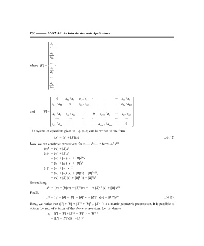
The system of equations given in Eq. (4.8) can be written in the form
{x} = {v} + [B]{x} ...(4.12)
(1)
(2)
Now we can construct expressions for x ... x ... in terms of x (0)
1
{x} = {v} + [B]x 0
2
{x} = {v} + [B]x l
= {v} + [B]({v} + [B]x )
(0)
2 0
= {v} + [B]({v} + [B] x )
3
{x} = {v} + [B]{x} (2)
= {v} + [B]({v} + [B]{v} + [B] x )
2 (0)
2
3 0
= {v} + [B]{v} + [B] {v} + [B] x
Generalizing
...
2
r–1
r (0)
(r)
x = {v} + [B]{v} + [B] {v} + + [B] {v} + [B] x
Finally
3 ...
2
(r) (0)
r–1
(r)
x = ([I] + [B] + [B] + [B] + [B] ){v} + [B] x ...(4.13)
3
r–1
2
Here, we notice that ([I] + [B] + [B] + [B] ... [B] ) is a matrix geometric progression. It is possible to
obtain the sum of r terms of the above expressions. Let us denote
3 ...
2
s = [I] + [B] + [B] + [B] + [B] r–1
r
r
= ([I] – [B] )([I] – [B]) –1