Page 220 - MATLAB an introduction with applications

Numerical Methods ——— 205

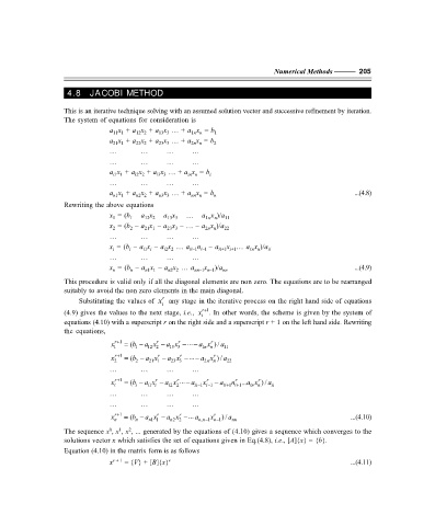
4.8 JACOBI METHOD

This is an iterative technique solving with an assumed solution vector and successive refinement by iteration.
The system of equations for consideration is
a x + a x + a x … + a x = b 1
11 1
1n n
13 3
12 2
a x + a x + a x … + a x = b 2
2n n
22 2
23 3
21 1
… … … …
… … … …
a x + a x + a x … + a x = b i
i3 3
i2 2
in n
i1 1
… … … …
a x + a x + a x … + a x = b n ...(4.8)
n2 2
nn n
n1 1
n3 3
Rewriting the above equations
x = (b – a x – a x – … – a x )/a 11
1
13 3
1n n
1
12 2
x = (b – a x – a x – … – a x )/a 22
2
2
2n n
21 1
23 3
… … … …
x … a x )/a
x = (b – a x – a x … a ii–1 i–1 – a ii+1 i+1 in n ii
n
i1 i
i
i2 2
i
… … … …
x = (b – a x – a x … a nn–1 n–1 )/a nn ...(4.9)
x
n2 2
n1 1
n
n
This procedure is valid only if all the diagonal elements are non zero. The equations are to be rearranged
suitably to avoid the non zero elements in the main diagonal.
r
Substituting the values of x any stage in the iterative process on the right hand side of equations
i
(4.9) gives the values to the next stage, i.e., x i r+ 1 . In other words, the scheme is given by the system of
equations (4.10) with a superscript r on the right side and a superscript r + 1 on the left hand side. Rewriting
the equations,
r
r
... ax
x 1 r+ 1 = (b − ax − a x − − 1nn r )/ a 11
1
13 3
12 2
r
r
x r+ 1 = (b − a x − a x − − 2nn r )/ a 22
... a x
23 3
21 1
2
2
… … … …
r
r
r
−
n
x i r+ 1 = (b − a x − a x r ... a ii− 1 i− 1 − a ii+ 1 i+ 1 ...a x r ) / a ii
x
in n
i
1 i
i
i
2 2
… … … …
… … … …
r
r
r
x
x r+ 1 = (b − a x − a x − ... a , n n− 1 n− 1 )/ a nn ...(4.10)
n
n
n
n
2 2
11
1
2
0
The sequence x , x , x , ... generated by the equations of (4.10) gives a sequence which converges to the
solutions vector x which satisfies the set of equations given in Eq.(4.8), i.e., [A]{x} = {b}.
Equation (4.10) in the matrix form is as follows
x r + 1 = {V} + [B]{x} r ...(4.11)