Page 266 - MATLAB an introduction with applications

Numerical Methods ——— 251

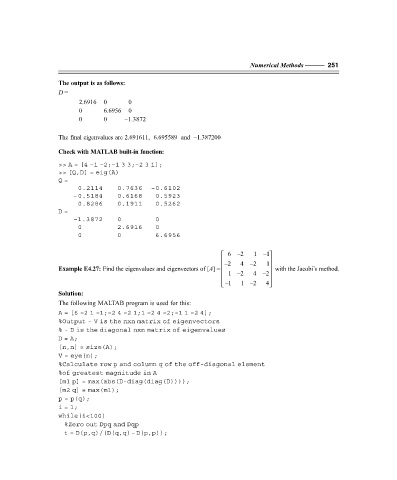
The output is as follows:
D =
2.6916 0 0
0 6.6956 0
0 0 –1.3872

The final eigenvalues are 2.691611, 6.695589 and –1.387200

Check with MATLAB built-in function:
>> A = [4 –1 –2;–1 3 3;–2 3 1];
>> [Q,D] = eig(A)
Q =
0.2114 0.7636 –0.6102
–0.5184 0.6168 0.5923
0.8286 0.1911 0.5262
D =
–1.3872 0 0
0 2.6916 0
0 0 6.6956

 6–2 1–1
 –2 4 –2 1 
Example E4.27: Find the eigenvalues and eigenvectors of [A] =   with the Jacobi’s method.
 1–2 4 –2
 
  –1 1 –2 4 
Solution:
The following MALTAB program is used for this:
A = [6 –2 1 –1;–2 4 –2 1;1 –2 4 –2;–1 1 –2 4];
%Output - V is the nxn matrix of eigenvectors
% - D is the diagonal nxn matrix of eigenvalues
D = A;
[n,n] = size(A);
V = eye(n);
%Calculate row p and column q of the off-diagonal element
%of greatest magnitude in A
[m1 p] = max(abs(D-diag(diag(D))));
[m2 q] = max(m1);
p = p(q);
i = 1;
while(i<100)
%Zero out Dpq and Dqp
t = D(p,q)/(D(q,q)–D(p,p));