Page 265 - MATLAB an introduction with applications

250 ——— MATLAB: An Introduction with Applications

Check with MATLAB built-in function:
>> A = [4 2 0 0; 2 8 2 0; 0 2 8 2; 0 0 2 4]; b = [4;0;0;14];
>> x = A\b
x =
1.0000
0
–1.0000
4.0000
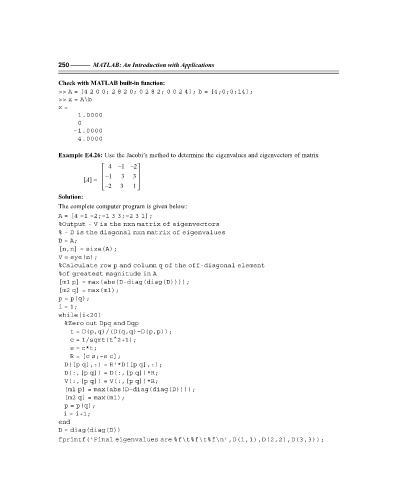
Example E4.26: Use the Jacobi’s method to determine the eigenvalues and eigenvectors of matrix
 4 –1 –2
 –1 3 3 
[A] =  
  –2 3 1 
Solution:
The complete computer program is given below:
A = [4 –1 –2;–1 3 3;–2 3 1];
%Output - V is the nxn matrix of eigenvectors
% - D is the diagonal nxn matrix of eigenvalues
D = A;
[n,n] = size(A);
V = eye(n);
%Calculate row p and column q of the off-diagonal element
%of greatest magnitude in A
[m1 p] = max(abs(D-diag(diag(D))));
[m2 q] = max(m1);
p = p(q);
i = 1;
while(i<20)
%Zero out Dpq and Dqp
t = D(p,q)/(D(q,q)–D(p,p));
c = 1/sqrt(t^2+1);
s = c*t;
R = [c s;–s c];
D([p q],:) = R'*D([p q],:);
D(:,[p q]) = D(:,[p q])*R;
V(:,[p q]) = V(:,[p q])*R;
[m1 p] = max(abs(D–diag(diag(D))));
[m2 q] = max(m1);
p = p(q);
i = i+1;
end
D = diag(diag(D))
fprintf(‘Final eigenvalues are %f\t%f\t%f\n’,D(1,1),D(2,2),D(3,3));