Page 263 - MATLAB an introduction with applications

248 ——— MATLAB: An Introduction with Applications

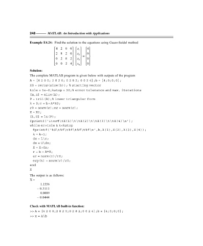
Example E4.24: Find the solution to the equations using Gauss-Seidel method

 4200   4
x
1
 28 2 0   
x


0 
   =  
2
 02 8 2   
0
x
3
 

x
 
  00 24    0 
4
Solution:
The complete MATLAB program is given below with outputs of the program
A = [4 2 0 0; 2 8 2 0; 0 2 8 2; 0 0 2 4];b = [4;0;0;0];
X0 = zeros(size(b)); % starting vector
tole = 1e-6;kstop = 30;% error tolerance and max. iterations
[n,n] = size(A);
P = tril(A);% lower triangular form
k = 0;r = b–A*X0;
r0 = norm(r);er = norm(r);
X = X0;
[L,U] = lu(P);
fprintf(‘iter#\tX(1)\t\tX(2)\t\tX(3)\t\tX(4)\n’);
while er>tole & k<kstop
fprintf(‘%d\t%f\t%f\t%f\t%f\n’,k,X(1),X(2),X(3),X(4));
k = k+1;
dx = L\r;
dx = U\dx;
X = X+dx;
r = b – A*X;
er = norm(r)/r0;
erp(k) = norm(r)/r0;
end
X
The output is as follows:
X =
1.1556
– 0.3111
0.0889
– 0.0444

Check with MATLAB built-in function:
>> A = [4 2 0 0;2 8 2 0;0 2 8 2;0 0 2 4];b = [4;0;0;0];
>> x = A\b