Page 267 - MATLAB an introduction with applications

252 ——— MATLAB: An Introduction with Applications

c = 1/sqrt(t^2+1);
s = c*t;
R = [c s;– s c];
D([p q],:) = R’*D([p q],:);
D(:,[p q]) = D(:,[p q])*R;
V(:,[p q]) = V(:,[p q])*R;
[m1 p] = max(abs(D-diag(diag(D))));
[m2 q] = max(m1);
p = p(q);
i = i+1;
end
D = diag(diag(D))
fprintf(‘Eigenvectors are\n’)
disp(V)

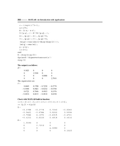
The output is as follows:
D =
9.1025 0 0 0
0 1.5186 0 0
0 0 4.5880 0
0 0 0 2.7910
The eigenvectors are
V =
0.6043 0.1788 – 0.7250 – 0.2778
– 0.5006 0.5421 – 0.0252 – 0.6744
0.4721 0.7046 0.4915 0.1976
– 0.4016 0.4215 – 0.4818 0.6550

Check with MATLAB built-in function:
>> A = [6 –2 1 –1;–2 4 –2 1;1 –2 4 –2;–1 1 –2 4];
>> [Q,D] = eig(A)
Q =
–0.1788 –0.2778 0.7250 –0.6043
–0.5421 –0.6744 0.0252 0.5006
–0.7046 0.1976 –0.4915 –0.4721
–0.4215 0.6550 0.4818 0.4016
D =
1.5186 0 0 0
0 2.7910 0 0
0 0 4.5880 0
0 0 0 9.1025