Page 312 - MATLAB an introduction with applications

Optimization ——— 297

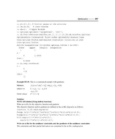
>> x0=[–1,1]; % Initial guess at the solution
>> lb=[0,0]; % Lower bounds
>> ub=[]; % Upper bounds
>> options=optimset(‘LargeScale’, ‘off’);
>> [x,fval]=fmincon(@objfun,x0,[],[],[],[],lb,ub,@confun,options)
Optimization terminated: first-order optimality measure less
than options.TolFun and maximum constraint violation is less
than options.TolCon.
Active inequalities (to within options.TolCon = 1e–006):
lower upper ineqlin ineqnonlin
1 1
x =
0 1.5000
fval =
8.5000
>> [c,ceq]=confun(x)
c =
0
–10
ceq =
[]

Example E5.18: This is a constrained example with gradients.
2
2
Minimize f ( ) x = e 1 x (4x + 2x + 4x x + 2x + 0.9)
2
1
2
1 2
subject to 2 + x x – x – x ≤ 0
1
1 2
2
–x x ≤ 0
1 2
0
Initial values: x = [–1, 1].
Solution:
MATLAB Solution [Using built-in function]:
Write an m-file for the objective function and gradient:
The objective function and its gradient are defined in the m-file objgrad.m as follows:
function [f,G]=objfungrad(x)
f=exp (x(1))*(4*x(1)^2+2*x(2)^2+4*x(1)*x(2)+2*x(2)+0.9);
t=exp(x(1))*(4*x(1)^2+2*x(2)^2+4*x(1)*x(2)+2*x(2)+0.9);
G=[t+exp(x(1))*(8*x(1)+4*x(2)),
exp(x(1))*(4*x(1)+4*x(2)+2)];
Write an m-file for the nonlinear constraints and the gradients of the nonlinear constraints:
The constraints and their partial derivatives are contained in the m-file confungrad.m: