Page 313 - MATLAB an introduction with applications

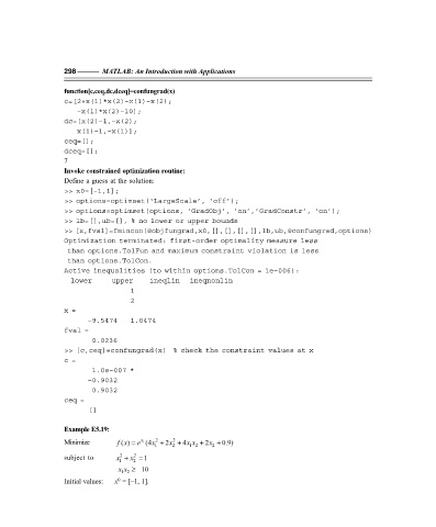
298 ——— MATLAB: An Introduction with Applications

function[c,ceq,dc,dceq]=confungrad(x)
c=[2+x(1)*x(2)–x(1)–x(2);
–x(1)*x(2)–10];
dc=[x(2)–1,–x(2);
x(1)–1,–x(1)];
ceq=[];
dceq=[];
7
Invoke constrained optimization routine:
Define a guess at the solution:
>> x0=[–1,1];
>> options=optimset(‘LargeScale’, ‘off’);
>> options=optimset(options, ‘GradObj’, ‘on’,’GradConstr’, ‘on’);
>> lb=[],ub=[], % no lower or upper bounds
>> [x,fval]=fmincon(@objfungrad,x0,[],[],[],[],lb,ub,@confungrad,options)
Optimization terminated: first-order optimality measure less
than options.TolFun and maximum constraint violation is less
than options.TolCon.
Active inequalities (to within options.TolCon = 1e–006):
lower upper ineqlin ineqnonlin
1
2
x =
–9.5474 1.0474
fval =
0.0236
>> [c,ceq]=confungrad(x) % check the constraint values at x
c =
1.0e–007 *
–0.9032
0.9032
ceq =
[]

Example E5.19:
2
2
x
Minimize f () = e 1 x (4x + 2x + 4x x + 2x + 0.9)
2
1
2
1 2
2
2
subject to x + x = 1
1
2
–x x ≥ –10
1 2
Initial values: x = [–1, 1].
0