Page 335 - MATLAB an introduction with applications

320 ——— MATLAB: An Introduction with Applications

to derivatives. Hence, the general differential equation such as (6.1) and the associated boundary conditions,
if any, are replaced by the corresponding finite difference equations. The continuous variable t is replaced
by the discrete variable t and the differential equation is solved progressively in time increments h = ∆ t
i
starting from known initial conditions. The solution obtained is approximate but by suitably selecting the
time increment the accuracy of the solution can be improved.

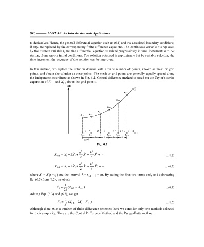
In this method, we replace the solution domain with a finite number of points, known as mesh or grid
points, and obtain the solution at these points. The mesh or grid points are generally equally spaced along
the independent coordinate as shown in Fig. 6.1. Central difference method is based on the Taylor’s series
expansion of X and X i–1 about the grid point i.
i+1
x(t)
x(t)
x i+3
x i+2

x i+1
x i
x i–1
x i–2

i–1 i–2 i i+1 i+2 i+3
t
0 t i–2 t i–1 t i t i+1 t i+2 t i+3
h h h h
∆t=h
Fig. 6.1

X = X + hX + h 2 X + h 3 + ... ...(6.2)
X
i
i
+ i
1
2 i 6 i
X
X = X − hX + h 2 X − h 3 . i + ... ... (6.3)
− i
1
i
i
2 i 6
( = t and the interval h
where X i = X t i ) = t + i 1 − t i = ∆t. By taking the first two terms only and subtracting
Eq. (6.3) from (6.2), we obtain
X = 1 (X − X ) ...(6.4)
i
2h + i 1 − i 1
Adding Eqs. (6.3) and (6.2), we get

X = 1 (X i− 1 − 2X + X i+ 1 ) ...(6.5)
i
i
h 2
Although there exist a number of finite difference schemes, here we consider only two methods selected
for their simplicity. They are the Central Difference Method and the Runge-Kutta method.