Page 339 - MATLAB an introduction with applications

324 ——— MATLAB: An Introduction with Applications

X i–1 X i X i+1

∆t ∆t
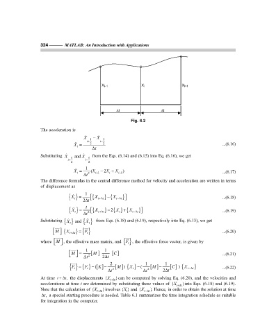
Fig. 6.2
The acceleration is

X 1 − X 1
i+ i−

X = 2 2 ...(6.16)
i
∆t
Substituting X 1 and X 1 from the Eqs. (6.14) and (6.15) into Eq. (6.16), we get
i+ i−
2 2

X = 1 (X − 2X + X ) ...(6.17)
i
∆t 2 i+ 1 i i− 1
The difference formulas in the central difference method for velocity and acceleration are written in terms
of displacement as
1

{ } = 2 t ∆   {X t+ ∆ } {X t− ∆t t  ...(6.18)
−
}
X
t

−
{ } = t 2   {X t+ ∆ } 2 X t + t− ∆t t  ...(6.19)
}
X
{ } {X
t
∆t

Substituting X t { } from Eqs. (6.18) and (6.19), respectively into Eq. (6.13), we get
{ } and X
t
M   { X t+ ∆t } {} ...(6.20)

=
F

t

F
where M  , the effective mass matrix, and {} , the effective force vector, is given by


t
1
1
  M  = ∆t 2 [ ] 2 t ∆ [] ...(6.21)
C
M

2 1 1
F −
{} {} [] − [ ] { } − ( [ ] − [] {X t− ∆t } ...(6.22)
F =
M
) X
)
C
M
( K
t
t
t
∆ 2 ∆t t 2 2 t ∆
At time t +∆ the displacements {X t+∆ t }can be computed by solving Eq. (6.20), and the velocities and
, t
accelerations at time t are determined by substituting these values of {X t+∆ t }into Eqs. (6.18) and (6.19).
Note that the calculation of {X t+∆ t }involves {X } and {X – t ∆ t } . Hence, in order to obtain the solution at time
t
, t ∆ a special starting procedure is needed. Table 6.1 summarizes the time integration schedule as suitable
for integration in the computer.