Page 343 - MATLAB an introduction with applications

328 ——— MATLAB: An Introduction with Applications

=
y
{ t+ ∆t } { } ∆ (y + t aK + bK + cK + dK 4 ) ...(6.40)
3
1
2
t
where a, b, c and d are constants and K K , K and K are the approximate derivative values computed in
3
2
1,
4
t
the interval t K << t K+ ∆t . Several fourth order algorithms have been proposed. The following is due to
Runge-Kutta and we omit presenting the details of its derivation.
∆t
=
y
y
{ t+ ∆t } { } + [K + 2K + 2K + K 4 ] ...(6.41)
2
t
3
1
6
K = f (, )
t
y
t
1

K = f t + ∆ 2 , y + K 1 ∆t 2 t  


2
t

in which K = f t + ∆ 2 , y + K 2 ∆t 2 t    ...(6.42)


t
3
K = ( f t + ∆ , t y + K 3 ∆ ) t
t
4
The Runge-Kutta algorithm does not require the calculation of higher derivatives. This method is completely
self-starting and the step size can be changed easily between iterations and hence the method can be
considered inherently stable. The truncation error e for the fourth-order Runge-Kutta scheme is of the form
t
e = ct 5 ...(6.43)
∆
( )
t
where c is constant, which depends on f (t , y) and its higher-order partial derivatives. Runge-Kutta method
generates an artificial damping that unduly suppresses the amplitude of the response of a dynamic system
to some extent.
6.5 IMPLICIT SCHEMES
In an implicit scheme, the difference equations are combined with the equations of motion, and the
displacements are calculated directly by solving the equations.
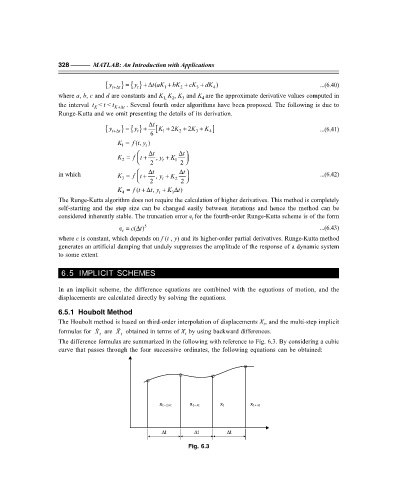
6.5.1 Houbolt Method
The Houbolt method is based on third-order interpolation of displacements X , and the multi-step implicit
t

formulas for X are X obtained in terms of X by using backward differences.
t
t
t
The difference formulas are summarized in the following with reference to Fig. 6.3. By considering a cubic
curve that passes through the four successive ordinates, the following equations can be obtained:
x t–2 t∆ x t– t∆ x t x t+ t∆
∆t ∆t ∆t
Fig. 6.3