Page 345 - MATLAB an introduction with applications

330 ——— MATLAB: An Introduction with Applications

required displacements X t+ ∆t . The term KX t+ ∆t appears because the equilibrium is considered at time t + t∆
and not at time t as in the central difference method. There is no critical time-step limit, and t∆ can in
general be selected much larger than that given for the central difference method.

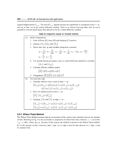
Table 6.3 Algorithm based on Houbolt method
(a) Initial Computations:
1. Form stiffness [K], mass [M] and damping [C] matrices
2. Initialize { } { } and X 0

{ } .
, X
X
0
0
3. Select time step t∆ and calculate integration constants:
2 11 5 3 − a
a = ; a = ; a = ; a = ; a = − 2 ; a = 3 ;
a
∆ 0 2 1 6 t ∆ 2 ∆t t 2 3 ∆t 4 0 5 2
a a
a = 0 ; a = 3 .
6
2 7 9
4. Use special starting procedure, such as central-difference method to calculate.
{
{X ∆t } and X 2 t ∆ }.
5. Calculate effective stiffness matrix:
 [] a M+ [ ] a C+ [ ]
K =
K
 0 1
 
L
D
L
6. Triangularize K : K = [] [ ] [ ] T
 
(b) For each time step:
1. Calculate effective force vector at time t + t∆ :
+
+
+
F = F } [ ] (a { } a {X } a {X })
M
X
{ t+ ∆ } { t+ ∆t t 2 t 4 t− ∆t 6 t− 2 t ∆
+ [] (C a 3 { } a 5 {X t− ∆t } a 7 {X t− 2 t ∆ })
+
+
X
t
2. Solve for displacements at time t + t∆
 {X t+ ∆  } { t+ ∆t t }
=
F
K

X
3. Calculate {} and X {} at time t + t∆ :
−
−
−
{ X t+ ∆t } = a 1 {X t+ ∆t } a 3 { } a 5 {X t− ∆t } a 7 {X t− 2 t ∆ }
X
t

−
−
−
{ X t+ ∆t } = a 0 {X t+ ∆t } a 2 { } a 4 {X t− ∆t } a 6 {X t− 2 t ∆ }
X
t
6.5.2 Wilson Theta Method
The Wilson Theta Method assumes that the acceleration of the system varies linearly between two instants
of time. Referring to Fig. 6.4, the acceleration is assumed to be linear from time t between , t = i t∆ to time
i
t i+θ =+ θ∆ t , where θ≥ 1.0 . Because of this reason, the method is known as the Wilson Theta method.
t
i
If τ is the increase in time t between t and t + θ∆ ( 0 ≤τ ≤ θ∆ ), then for time interval t to t + θ∆ , it can
t
t
t
be assumed that