Page 349 - MATLAB an introduction with applications

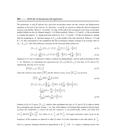
334 ——— MATLAB: An Introduction with Applications

The parameters α and β indicate how much the acceleration enters into the velocity and displacement
equations at the end of the interval ∆t. Therefore, α and β are chosen to obtain the desired integration
accuracy and stability. When α =1/6 and β =1/2, Eqs. (6.69) and (6.70) correspond to the linear acceleration
method (which can also be obtained using θ =1 in Wilson method). When α =1/2 and β = 0, the acceleration

is constant and equal to X during each time interval ∆t. If α = 1/2 and β = 1/8, the acceleration is constant
t

from the beginning as X and then changes to X t+∆ t in the middle of the time interval ∆t. When α = 1/2 and
t
β = 1/4, this corresponds to the assumption that the acceleration remains constant at an average value of

(X + X t+ ∆t )/2 . The finite difference formulas for the Newmark Beta scheme are
t

−
{ X t+ ∆ } = 1 { ( X t+ ∆t t } { }) − 1 { } −   1 − 1   { } ...(6.71)
X
X
X
t
t
t
β∆t 2 β∆t  2β 
α
α

−
−
X
X
X
{ X t+ ∆ } = β α { ( X t+ ∆t t } { }) −   β − 1    { } ∆t    2β − 1    { } ...(6.72)
t
t
t
∆t
Equation (6.13) can be employed to obtain a solution for displacements, velocity and accelerations at time
{
t + ∆t. Therefore, by substituting the expressions for { X t+ ∆ } and X t+ ∆t t } from Eqs. (6.71) and (6.72),
respectively, into Eq. (6.13), we get
M   {X t+ ∆  } { t+ ∆t t } ...(6.73)

=
F

F


where the effective mass matrix M  and the effective force vector { t+ ∆t } are given by
 M  = 1 M α [] [ ]
C +
K
  β ∆t 2 [ ] + β ∆t ...(6.74)
 1   α  

X
{ F t+ ∆t = F ∆t } +  − 1 M +  − 1  [] { }
C
[ ] ∆t


} { t+
t
2
 β   2β  
 1  α  
[] { }
M +
+  [ ]  − 1 C  X t

 β ∆t β  
 1 α 
+  2 [ ] + [] { } ...(6.75)
X
M
C

t
 β∆t β ∆t 
Solution of Eq. (6.73) gives {X t+ ∆t } , which is then substituted into Eqs. (6.71) and (6.72) in order to obtain
the accelerations and velocities at time t + t∆ . One of the features of Newmark Beta method is that for linear
systems the amplitude is conserved and the response is unconditionally stable, provided that
1 1  1 2 1 1
α≥ and β ≥  α+  . For values of α= and β= , the largest truncation errors occur in the
2 4  2  2 4
1
frequency of the response as opposed to other β values. It is also important to note that unless β= ,
2
1
there is a spurious damping introduced, proportional to β− . If β = 0, a negative damping results; this
2