Page 347 - MATLAB an introduction with applications

332 ——— MATLAB: An Introduction with Applications

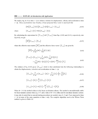
We employ Eq. (6.13) at time t + t∆ to obtain a solution for displacement, velocity and acceleration at time
t + t∆ . Since accelerations vary linearly, a linear projected force vector is used such that

=
+
+
[ ]{ X t+ θ∆t } []{ X t+ θ∆t } []{X t+ θ∆t } { t+ θ∆t } ...(6.62)
C
K
F
M
=
−
F
where { t+ θ∆t } {} θ (F + ∆ t F θ∆t }{})F t .
{ t+
t
{
By substituting the expressions for { X t+ θ∆t } and X t+ θ∆t } from Eqs. (6.60) and (6.61), respectively, into
Eq.(6.62), we get
 M  {X = F } ...(6.63)
  t+ θ∆t } { t+∆ t
 F


where the effective mass matrix M  and the effective force vector { t+∆ t } are given by
6
3

C +
M  = θ∆t 2 [ ] + θ∆t [] [ ] (6.64)
K
M


2
6 3
+
M
) X
C
{ F t+ θ∆t = F θ∆t } ( [ ] + [] { }
t
} { t+
2
θ∆t 2 θ∆t
6 θ∆t (6.65)

+
M +
[ ] { } (2 M +
C
) X
( [ ] 2 C ) X + [ ] [] { }
θ∆t t 2 t
The solution of Eq. (6.63) gives {X t+ θ∆t } which is then substituted into the following relationships to
obtain the displacements, velocities and accelerations at time t + t∆ .
3

−
{ X t+ ∆ } = 6 { ( X t+ θt ∆ t } { }) − 6 { } +   1−  { } ...(6.66)
X
X
X
t
t
t
2
2
θ∆t 2 θ∆t  θ 

−
=
{ X t+ ∆ } { } + ∆t { ( X t+ ∆t t } { } )X t ...(6.67)
X
t
2

−
{ } +
=
2
{X t+ ∆ } { } ∆X t + t X t ∆t 2 { ( X t+ ∆t t } { })X t ...(6.68)
6
When θ = 1.0, the method reduces to the linear acceleration scheme. The method is unconditionally stable
for linear dynamic systems when θ≥ 1.37, and a value of θ =1.4 is often used for non-linear dynamic systems.

It may also be noted that no special starting procedures are needed, since X, X and X are expressed at time
t + t∆ in terms of the same quantities at time t only. The complete algorithm used in the Wilson Theta
method is given in Table 6.4.