Page 350 - MATLAB an introduction with applications

Direct Numerical Integration Methods ——— 335

involves a self-excited vibration arising solely from the numerical procedure. In a likewise manner, if β is
1
greater than , a positive damping is introduced which reduces the magnitude of the response even without
2
real damping in the problem. For a multi-degree of freedom system in which a number of modes constitute
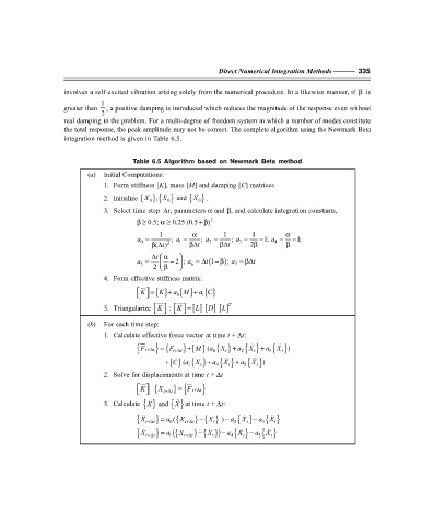
the total response, the peak amplitude may not be correct. The complete algorithm using the Newmark Beta
integration method is given in Table 6.5.

Table 6.5 Algorithm based on Newmark Beta method
(a) Initial Computations:
1. Form stiffness [K], mass [M] and damping [C] matrices
2. Initialize { } { } and X 0

, X
{ } .
X
0
0
3. Select time step t∆ , parameters α and β, and calculate integration constants,
β≥ 0.5; α ≥ 0.25 (0.5+β ) 2
1 α 1 1 α
a = ; a = ; a = ; a = − 1; a = − 1;
0
β∆ ) 2 1 β∆ t 2 β∆ t 3 2β 4 β
( t
∆ t  α 
a = 2 β − 2; a = ( t ∆ 1− β ); a = β∆ t


5
6
7

4. Form effective stiffness matrix:
 [] a M+ 0 [ ] a C+ 1 [ ]
K =
K




D
5. Triangularize K : K = [] [ ] [] L T
L


(b) For each time step:
1. Calculate effective force vector at time t + t∆ :

+
+
+
M
{ F t+ ∆t = F ∆t } [ ] (a 0 { } a 2 { } a 3 { } )X t
X
X
} { t+
t
t

+ [] (C a X t + 4 { } a 5 { } )X t
+
X
{ } a
t
1
2. Solve for displacements at time t + t∆
 {X t+ ∆t } { F t+ ∆t }
=
K


X
3. Calculate {} and X {} at time t + t∆ :

−
−
X
) a
X
{ X t+ ∆t } = a 0 { ( X t+ ∆t } { } − 2 { } a 3 { }
X
t
t
t

−
−
−
X
{ X t+ ∆t } = a 1 { ( X t+∆ t } { }) a 4 { } a 5 { }
X
X
t
t
t