Page 355 - MATLAB an introduction with applications

340 ——— MATLAB: An Introduction with Applications

1.4

1.2

1
Displacement(m) 0.8

0.6

0.4

0.2

0
0 1 2 3 4 5 6
Time(s)
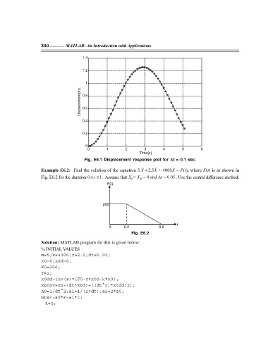
Fig. E6.1 Displacement response plot for ∆∆ ∆∆ ∆t = 0.1 sec.

Example E6.2: Find the solution of the equation 5 X + 2.5X + 4000X = F(t), where F(t) is as shown in

Fig. E6.2 for the duration 0 t≤≤ 1. Assume that X = X = 0 and ∆t = 0.05 . Use the central difference method.
0
0
F(t)

200

t
0 0.2 0.6
Fig. E6.2

Solution: MATLAB program for this is given below:
% INITIAL VALUES
m=5;k=4000;c=2.5;dt=0.05;
x0=0;x0d=0;
F0=200;
T=1;
x0dd=inv(m)*(F0-c*x0d-k*x0);
xprev=x0-(dt*x0d)+((dt^2)*x0dd/2);
a0=1/dt^2;a1=1/(2*dt);a2=2*a0;
mbar=a0*m+a1*c;
t=0;