Page 359 - MATLAB an introduction with applications

344 ——— MATLAB: An Introduction with Applications

end
for i=2:p-1
if i<p-1
v(i)=(X(i+1)-X(i-1))/(2*dt);
a(i)=(X(i+1)-2*X(i)+X(i-1))/dt^2;
end
end
fprintf(‘\ntime\t\tdisplacement\tvelocity\tacceleration\n’);
i=1;
for t=0:dt:T
fprintf(‘%f\t%f\t%f\t%f\n’,t,X(i),v(i),a(i));
i=i+1;
end
t=[0:dt:T+dt];
plot(t,X,‘-p’);
xlabel(‘time(s)’);
ylabel(‘displacement(m)’);
grid on;

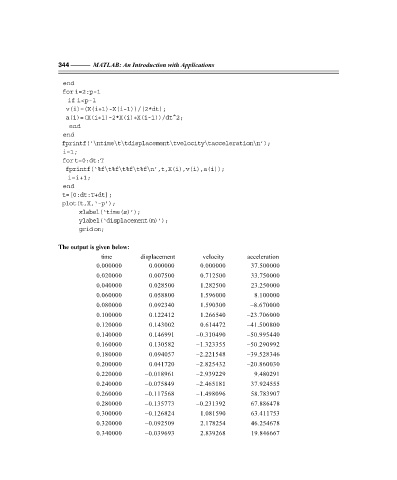
The output is given below:
time displacement velocity acceleration
0.000000 0.000000 0.000000 37.500000
0.020000 0.007500 0.712500 33.750000
0.040000 0.028500 1.282500 23.250000
0.060000 0.058800 1.596000 8.100000
0.080000 0.092340 1.590300 –8.670000
0.100000 0.122412 1.266540 –23.706000
0.120000 0.143002 0.614472 –41.500800
0.140000 0.146991 –0.310490 –50.995440
0.160000 0.130582 –1.323355 –50.290992
0.180000 0.094057 –2.221548 –39.528346
0.200000 0.041720 –2.825432 –20.860030
0.220000 –0.018961 –2.939229 9.480291
0.240000 –0.075849 –2.465181 37.924555
0.260000 –0.117568 –1.498096 58.783907
0.280000 –0.135773 –0.231392 67.886478
0.300000 –0.126824 1.081590 63.411753
0.320000 –0.092509 2.178254 46.254678
0.340000 –0.039693 2.839268 19.846667