Page 363 - MATLAB an introduction with applications

348 ——— MATLAB: An Introduction with Applications

The output is given below:
time displacement velocity acceleration
0.000000 0.000000 0.000000 0.000000
0.050000 0.000000 1.875000 75.000000
0.100000 0.187500 6.759780 120.391187
0.150000 0.675978 12.725905 118.253838
0.200000 1.460091 17.418045 69.431745
0.250000 2.417782 15.233816 –156.800902
0.300000 2.983472 3.285518 –321.131034
0.350000 2.746334 –13.709851 –358.683716
0.400000 1.612487 –29.042788 –254.633742
0.450000 –0.157945 –34.785091 24.941603
0.500000 –1.866022 –26.794791 294.670399
0.550000 –2.837424 –8.226331 448.067983
0.600000 –2.688655 13.589754 424.575418
0.650000 –1.478448 30.040819 233.467197
0.700000 0.315427 34.632244 –49.810180
0.750000 1.984776 25.551408 –313.423286
0.800000 2.870567 6.383280 –453.301838
0.850000 2.623104 –15.304866 –414.223998
0.900000 1.340081 –30.950893 –211.617078
0.950000 –0.471985 –34.377997 74.532916
1.000000 –2.097719 –24.233212 331.258494

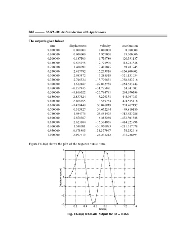
Figure E6.4(a) shows the plot of the response versus time.

3

2 1

Displacement(m) –1

0

–2

–3
0 0.2 0.4 0.6 0.8 1 1.2 1.4
Time(s)
Fig. E6.4 (a) MATLAB output for ∆∆ ∆∆ ∆t = 0.05s