Page 366 - MATLAB an introduction with applications

Direct Numerical Integration Methods ——— 351

0.900000 2.815997 3.558129 –9.544163
0.950000 2.981973 3.021179 –11.933829
1.000000 3.118115 2.371360 –14.058926
1.050000 3.219109 1.626489 –15.735916
1.100000 3.280764 0.812907 –16.807359
1.150000 3.300400 –0.036584 –17.172266
1.200000 3.277105 –0.886080 –16.807592
1.250000 3.211792 –1.700621 –15.774049
1.300000 3.107043 –2.450079 –14.204274
1.350000 2.966784 –3.112116 –12.277189
1.400000 2.795832 –3.673705 –10.186361
1.450000 2.599413 –4.131135 –8.110872
1.500000 2.382718 –4.488775 –6.194716
1.550000 2.150536 –4.757067 –4.536959
1.600000 1.907011 –4.950278 –3.191475
1.650000 1.655508 –5.084393 –2.173152
1.700000 1.398572 –5.175400 –1.467123
1.750000 1.137968 –5.238034 –1.038230
1.800000 0.874769 –5.284965 –0.839002
1.850000 0.609472 –5.326325 –0.815407
1.900000 0.342136 –5.369468 –0.910322
1.950000 0.072525 –5.418854 –1.065097
2.000000 –0.199749 –5.475975 –1.219747
etc.

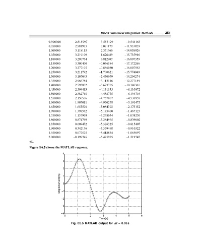
Figure E6.5 shows the MATLAB response.
4

3

2

Displacement(m) –1
1
0

–2
–3

–4
0 1 2 3 4 5 6
Time(s)
Fig. E6.5 MATLAB output for ∆∆ ∆∆ ∆t = 0.05s