Page 367 - MATLAB an introduction with applications

352 ——— MATLAB: An Introduction with Applications

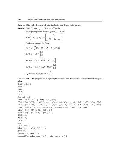
Example E6.6: Solve Example 6.1 using the fourth-order Runge-Kutta method.

Solution: Here Y = f (, , ) is a vector of functions
x
t
x
2
1
For single degree of freedom system, it contains
 x 2 
x



x

Y =  = f (, , ) =  1 
t
x
)
2
1
x
F
  m ( () t − kx − cx 2 
1


Final solution takes the form
t ∆
Y = Y + [K + 2K + 2K + K ], where
i
i+1
6 1 2 3 4

p
K = f (x , x , t) = 
1
2
1
q

r 
K = f (x + p/2, x + q/2, t + ∆t/2) = 
1
2
2
s


u
K = f (x + r/2, x + q/2, t + ∆t/2) = 
2
3
1
v


m
K = f (x + u, x + v, t + ∆t) = 
4
n
2
1

Complete MATLAB program for computing the response and its derivative in every time step is given
below:
dt=0.5;T=10;
h=dt;
x1=0;
x2=0;
i=1;
for t=0:h:T
f1=h*f(t,x1,x2); g1=h*g(t,x1,x2);
f2=h*f((t+h/2),(x1+f1/2),(x2+g1/2));g2=h*g((t+h/2),(x1+f1/2),(x2+g1/2));
f3=h*f((t+h/2),(x1+f2/2),(x2+g2/2));g3=h*g((t+h/2),(x1+f2/2),(x2+g2/2));
f4=h*f((t+h),(x1+f3),(x2+g3)); g4=h*g((t+h),(x1+f3),(x2+g3));
x1=x1+((f1+f4)+2*(f2+f3))/6.0;
x2=x2+((g1+g4)+2*(g2+g3))/6.0;
X(i)=x1;
Y(i)=x2;
i=i+1;
end
t=[0:h:T];
plot(t,X,‘-p’,t,Y,‘-*’);
grid on;
xlabel(‘time(s)’);
legend(‘displacement(m)’,‘velocity(m/s)’,2)