Page 368 - MATLAB an introduction with applications

Direct Numerical Integration Methods ——— 353

This program is executed with two other separate programs f.m and g.m given below:

% file f.m
function v1=f(t,x1,x2)
v1=x2;
% file g.m
function v2=g(t,x1,x2)
k=1; m=1; c=0;
F=100*(1-cos(t));
v2=(F-k*x1-c*x2)/m;
The output values of the data are presented below:
time displacement velocity
0.000000 0.000000 0.000000
0.500000 0.110437 0.411687
1.000000 0.379029 0.629789
1.500000 0.707386 0.653171
2.000000 1.004189 0.510442
2.500000 1.198540 0.253323
3.000000 1.249282 –0.052604
3.500000 1.149336 –0.338363
4.000000 0.924789 –0.541854
4.500000 0.629191 –0.616591
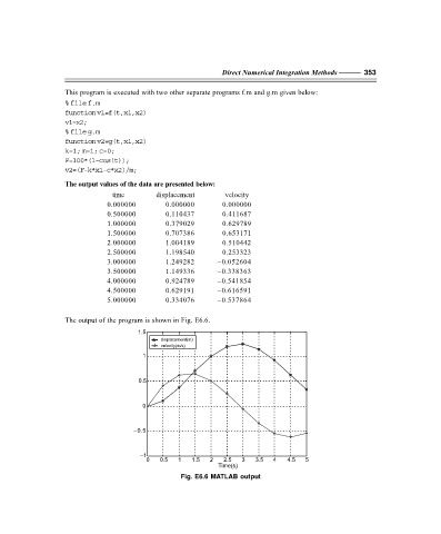
5.000000 0.334076 –0.537864

The output of the program is shown in Fig. E6.6.
1.5
displacement(m)
velocity(m/s)
1

0.5

0

–0.5

–1
0 0.5 1 1.5 2 2.5 3 3.5 4 4.5 5
Time(s)
Fig. E6.6 MATLAB output