Page 365 - MATLAB an introduction with applications

350 ——— MATLAB: An Introduction with Applications

xprev=x0;
x0=x;
i=i+1;
p=i;
end
for i=2:p-1
if i<p-1
v(i)=(X(i+1)-X(i-1))/(2*dt);
a(i)=(X(i+1)-2*X(i)+X(i-1))/dt^2;
end
end
fprintf(‘\ntime\t\tdisplacement\tvelocity\tacceleration\n’);
i=1;
for t=0:dt:T
fprintf(‘%f\t%f\t%f\t%f\n’,t,X(i),v(i),a(i));
i=i+1;
end
t=[0:dt:T+dt];
plot(t,X,’-p’);
xlabel(‘time(s)’);

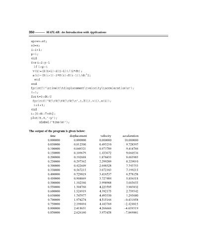
The output of the program is given below:
time displacement velocity acceleration
0.000000 0.000000 0.000000 10.000000
0.050000 0.012500 0.493210 9.728397
0.100000 0.049321 0.971789 9.414766
0.150000 0.109679 1.433672 9.060536
0.200000 0.192688 1.876835 8.665983
0.250000 0.297362 2.299209 8.229010
0.300000 0.422609 2.698528 7.743753
0.350000 0.567215 3.072103 7.199215
0.400000 0.729819 3.416537 6.578158
0.450000 0.908869 3.727404 5.856518
0.500000 1.102560 3.998908 5.003655
0.550000 1.308760 4.223595 3.983832
0.600000 1.524919 4.392175 2.759342
0.650000 1.747977 4.493550 1.295680
0.700000 1.974274 4.515166 –0.431058
0.750000 2.199494 4.443769 –2.424815
0.800000 2.418651 4.266666 –4.659319
0.850000 2.626160 3.973458 –7.069001