Page 369 - MATLAB an introduction with applications

354 ——— MATLAB: An Introduction with Applications

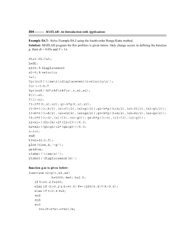
Example E6.7: Solve Example E6.2 using the fourth-order Runge-Kutta method.
Solution: MATLAB program for this problem is given below. Only change occurs in defining the function
g. Here dt = 0.05s and T = 1s.

dt=0.05;T=1;
h=dt;
x1=0; % displacement
x2=0; % velocity
i=1;
fprintf(‘time\t\tdisplacement\tvelocity\n’);
for t=0:h:T
fprintf(‘%f\t%f\t%f\n’,t,x1,x2);
X(i)=x1;
Y(i)=x2;
f1=h*f(t,x1,x2); g1=h*g(t,x1,x2);
f2=h*f((t+h/2),(x1+f1/2),(x2+g1/2));g2=h*g((t+h/2),(x1+f1/2),(x2+g1/2));
f3=h*f((t+h/2),(x1+f2/2),(x2+g2/2));g3=h*g((t+h/2),(x1+f2/2),(x2+g2/2));
f4=h*f((t+h),(x1+f3),(x2+g3)); g4=h*g((t+h),(x1+f3),(x2+g3));
x1=x1+((f1+f4)+2*(f2+f3))/6.0;
x2=x2+((g1+g4)+2*(g2+g3))/6.0;
i=i+1;
end
time=[0:h:T];
plot(time,X,‘–p’);
grid on;
xlabel(‘time(s)’);
ylabel(‘displacement(m)’)

function g.m is given below:

function v2=g(t,x1,x2)
k=4000; m=5; c=2.5;
if t<=0.2 F=200;
else if (t>0.2 & t<=0.6) F=–(200/0.4)*(t–0.6);
else if t>0.6 F=0;
end
end
end
v2=(F–k*x1–c*x2)/m;