Page 374 - MATLAB an introduction with applications

Direct Numerical Integration Methods ——— 359

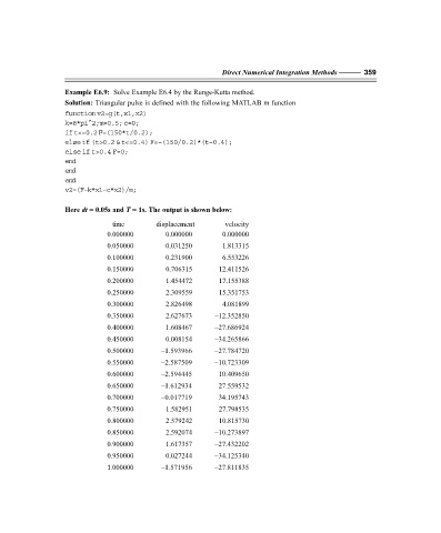
Example E6.9: Solve Example E6.4 by the Runge-Kutta method.
Solution: Triangular pulse is defined with the following MATLAB m function
function v2=g(t,x1,x2)
k=8*pi^2;m=0.5; c=0;
if t<=0.2 F=(150*t/0.2);
else if (t>0.2 & t<=0.4) F=–(150/0.2)*(t–0.4);
else if t>0.4 F=0;
end
end
end
v2=(F–k*x1–c*x2)/m;

Here dt = 0.05s and T = 1s. The output is shown below:
time displacement velocity
0.000000 0.000000 0.000000
0.050000 0.031250 1.813315
0.100000 0.231900 6.553226
0.150000 0.706315 12.411526
0.200000 1.454472 17.155388
0.250000 2.309559 15.351753
0.300000 2.826498 4.081899
0.350000 2.627673 –12.352850
0.400000 1.608467 –27.686924
0.450000 0.008154 –34.265866
0.500000 –1.593966 –27.784720
0.550000 –2.587509 –10.723309
0.600000 –2.594445 10.409650
0.650000 –1.612934 27.559532
0.700000 –0.017719 34.195743
0.750000 1.582951 27.798535
0.800000 2.579242 10.815730
0.850000 2.592074 –10.273897
0.900000 1.617357 –27.432202
0.950000 0.027244 –34.125340
1.000000 –1.571956 –27.811835