Page 375 - MATLAB an introduction with applications

360 ——— MATLAB: An Introduction with Applications

3

2

1
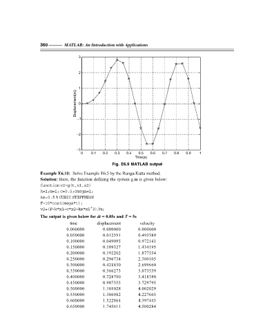
Displacement(m) 0

–1

–2

–3
0 0.1 0.2 0.3 0.4 0.5 0.6 0.7 0.8 0.9 1
Time(s)
Fig. E6.9 MATLAB output

Example E6.10: Solve Example E6.5 by the Runga-Kutta method.
Solution: Here, the function defining the system g.m is given below:
function v2=g(t,x1,x2)
k=1;m=1; c=0.5;omega=1;
ks=0.5 % CUBIC STIFFNESS
F=10*cos(omega*t);
v2=(F–k*x1–c*x2–ks*x1^3)/m;
The output is given below for dt = 0.05s and T = 5s
time displacement velocity
0.000000 0.000000 0.000000
0.050000 0.012391 0.493389
0.100000 0.049095 0.972141
0.150000 0.109327 1.434195
0.200000 0.192202 1.877534
0.250000 0.296734 2.300105
0.300000 0.421830 2.699660
0.350000 0.566273 3.073539
0.400000 0.728700 3.418380
0.450000 0.907555 3.729795
0.500000 1.101028 4.002029
0.550000 1.306982 4.227665
0.600000 1.522864 4.397443
0.650000 1.745611 4.500284