Page 364 - MATLAB an introduction with applications

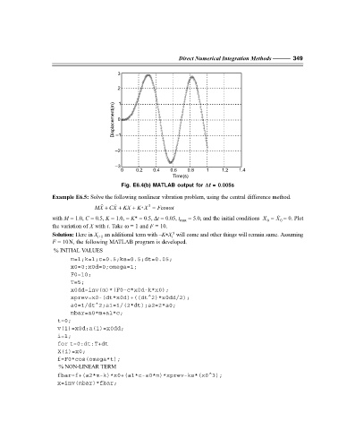
Direct Numerical Integration Methods ——— 349

3

2 1

Displacement(m) –1

0

–2

–3
0 0.2 0.4 0.6 0.8 1 1.2 1.4
Time(s)
Fig. E6.4(b) MATLAB output for ∆∆ ∆∆ ∆t = 0.005s

Example E6.5: Solve the following nonlinear vibration problem, using the central difference method.

3
MX + CX + KX + K X = F cosωt
∗

with M = 1.0, C = 0.5, K = 1.0, = K* = 0.5, ∆t = 0.05, t max = 5.0, and the initial conditions X = X = 0. Plot
0
0
the variation of X with t. Take ω = 1 and F = 10.
3
Solution: Here in X an additional term with –K*X will come and other things will remain same. Assuming
i+1
i
F = 10N, the following MATLAB program is developed.
% INITIAL VALUES
m=1;k=1;c=0.5;ks=0.5;dt=0.05;
x0=0;x0d=0;omega=1;
F0=10;
T=5;
x0dd=inv(m)*(F0-c*x0d-k*x0);
xprev=x0-(dt*x0d)+((dt^2)*x0dd/2);
a0=1/dt^2;a1=1/(2*dt);a2=2*a0;
mbar=a0*m+a1*c;
t=0;
v(1)=x0d;a(1)=x0dd;
i=1;
for t=0:dt:T+dt
X(i)=x0;
f=F0*cos(omega*t);
% NON-LINEAR TERM
fbar=f+(a2*m-k)*x0+(a1*c-a0*m)*xprev-ks*(x0^3);
x=inv(mbar)*fbar;