Page 356 - MATLAB an introduction with applications

Direct Numerical Integration Methods ——— 341

v(1)=x0d;a(1)=x0dd;
i=1;
for t=0:dt:T+dt
X(i)=x0;
if t<=0.2 f=F0;
else if (t>0.2 & t<=0.6) f=-(F0/0.4)*(t-0.6);
else if t>0.6 f=0;
end
end
end
fbar=f+(a2*m-k)*x0+(a1*c-a0*m)*xprev;
x=inv(mbar)*fbar;
xprev=x0;
x0=x;
i=i+1;
p=i;
end
for i=2:p-1
if i<p-1
v(i)=(X(i+1)-X(i-1))/(2*dt);
a(i)=(X(i+1)-2*X(i)+X(i-1))/dt^2;
end
end
fprintf(‘\ntime\t\tdisplacement\tvelocity\tacceleration\n’);
i=1;
for t=0:dt:T
fprintf(‘%f\t%f\t%f\t%f\n’,t,X(i),v(i),a(i));
i=i+1;
end
t=[0:dt:T+dt];
plot(t,X,‘-p’);
xlabel(‘time(s)’);
ylabel(‘displacement(m)’);
grid on;

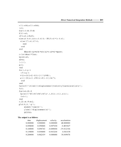
The output is as follows:
time displacement velocity acceleration
0.000000 0.000000 0.000000 40.000000
0.050000 0.050000 0.987654 –0.493827
0.100000 0.098765 –0.000000 –39.012346
0.150000 0.050000 –0.963268 0.481634
0.200000 0.002439 0.000000 38.049078