Page 352 - MATLAB an introduction with applications

Direct Numerical Integration Methods ——— 337

calculation of {X t+ ∆t } requires the displacements and velocities at t, t – t∆ and t –2 t∆ . Therefore, in order
to obtain the solution at time t∆ and 2 t∆ , a special starting procedure is needed, which makes the method
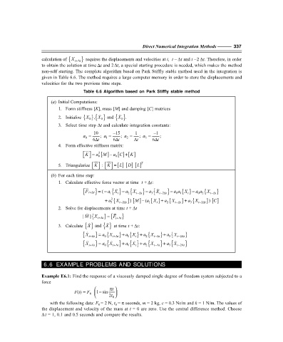
non-self starting. The complete algorithm based on Park Stiffly stable method used in the integration is
given in Table 6.6. The method requires a large computer memory in order to store the displacements and
velocities for the two previous time steps.

Table 6.6 Algorithm based on Park Stiffly stable method
(a) Initial Computations:
1. Form stiffness [K], mass [M] and damping [C] matrices

X
2. Initialize { } { } and X 0 , X 0 { }.
0
3. Select time step ∆t and calculate integration constants:
10 –15 1 –1
a = ; a = ; a = ; a = ;
0
∆
∆
∆
6 t 1 6 t 2 ∆t 3 6 t
4. Form effective stiffness matrix:
 a M − [ ] [ ]
K =
2
[ ] a C +
K
 0 0


D

L
5. Triangularize K : K = [] [ ] [] L T


(b) For each time step:
1. Calculate effective force vector at time t + t∆ :

−
−
−
( a X
{ } a a
{ F t+ ∆t } =− 1 { } a 2 { X t− ∆t } a 3 { X t− 2 t ∆ } a a X t − 0 2 {X t− ∆t }
t
0 1
+
+
{ } a
)
a 3 2 {X t−∆ } [ ] (M − a X t + 2 {X t− ∆t } a 3 {X t−∆ } []
) C
2 t
1
2 t
2. Solve for displacements at time t + t∆
=
| M { | X t+∆ t } { t+∆ t }
F

3. Calculate {} and X {} at time t + t∆ :
X
+
+
{ X t+ ∆t } = a 0 {X t+ ∆t } a X t + 2 {X t− ∆t } a 3 {X t− 2 t ∆ }
{ } a
1

+
+
{ } a
{ X t+ ∆t } = a 0 { X t+ ∆t } a X t + 2 { X t− ∆t } a 3 { X t− 2 t ∆ }
1
6.6 EXAMPLE PROBLEMS AND SOLUTIONS
Example E6.1: Find the response of a viscously damped single degree of freedom system subjected to a
force
 t π 
−
F(t) = F 1sin 2t  
0 

0
with the following data: F = 2 N, t = π seconds, m = 2 kg, c = 0.3 Ns/m and k = 1 N/m. The values of
0
0
the displacement and velocity of the mass at t = 0 are zero. Use the central difference method. Choose
∆t = 1, 0.1 and 0.5 seconds and compare the results.