Page 348 - MATLAB an introduction with applications

Direct Numerical Integration Methods ——— 333

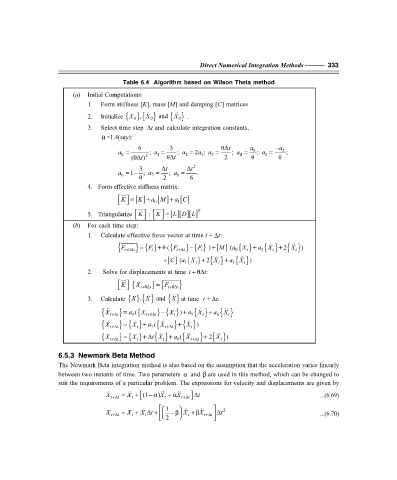
Table 6.4 Algorithm based on Wilson Theta method
(a) Initial Computations:
1. Form stiffness [K], mass [M] and damping [C] matrices

X
{ } .
, X
2. Initialize { } { } and X 0
0
0
3. Select time step t∆ and calculate integration constants,
θ =1.4(say):
6 3 θ∆t a − a
a = ; a = ; a = 2 ; a = ; a = 0 ; a = 2 ;
a
0
( ∆ ) tθ 2 1 θ∆t 2 1 3 2 4 θ 5 θ
3 ∆ ∆t t 2
a =− ; a = ; a = .
1
6
7
8
θ 2 6
4. Form effective stiffness matrix:
 [] a M+ 0 [ ] a C+ 1 [ ]
K =
K



L D
5. Triangularize K : K = [][ ][ ] L T


(b) For each time step:
1. Calculate effective force vector at time t + t∆ :

=
+
−
F
M
X
F
)
{ t+
{ t+ θ∆t } {} θF + ( F ∆t }{} + [ ] (a 0 { } a 2 { } { } )X t + 2 X t
t
t
t
+ [] (C a X 1 + 2 X t + 3 { } )X t
{ } { } a
1
2. Solve for displacements at time t +θ∆ t:
 { X t+θ ∆  } { t+θ ∆t t }
=
F
K

, X
X
3. Calculate {} {} and X
{} at time t + t∆ :

+
+
−
X
{ X t+ ∆t } = a 4 { ( X t+ θ∆t } { }) a 5 { } a 6 { }
X
X
t
t
t

+
+
=
X
X
{ X t+ ∆t } { } a 7 { ( X t+ ∆t } { } )
t
t

+
=
+
X
{ } a
{X t+ ∆t } { } ∆t X t + 8 { ( X t+ ∆t } { } )
2 X
t
t
6.5.3 Newmark Beta Method
The Newmark Beta integration method is also based on the assumption that the acceleration varies linearly
between two instants of time. Two parameters α and β are used in this method, which can be changed to
suit the requirements of a particular problem. The expressions for velocity and displacements are given by

X t+ ∆ = X +   (1− α )X + α X t+   ∆t ...(6.69)
t
t
t
∆t

X = X + X ∆  1 −β  X + β X t+   ∆t +   t 2 ...(6.70)
t+
t
t
∆
  2  t ∆t t 