Page 340 - MATLAB an introduction with applications

Direct Numerical Integration Methods ——— 325

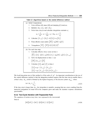
Table 6.1 Algorithms based on the central difference method
(a) Initial Computations:
1. Form stiffness [K], mass [M] and damping [C] matrices.

2. Initialize {X },{X 0 } and {{X 0 }.
0
3. Select time step ∆t and calculate integration constants a : i
1 1 1
a
a = 2 ; a = ; a = 2 ; a = .
0
2
1
3
0
∆
∆t 2 t a 2

=
{ } a
X
4. Calculate {X − ∆t } { } ∆X 0 − t X 0 + 3 { } .
0

[ ] a C+
5. Form effective mass matrix M  = a M 1 [ ] .


0
T


D
L
L
6. Triangularize M   : M  = [] [ ] [] .



(b) For each time step:
1. Calculate effective force vector at time t:
( K −
[ ] { } −
F =
F −
{} {} [] a M ) X t (a M − 1 [ ] {X t− ∆t }
)
[ ] a C
0
t
t
2
2. Solve for displacements at time t +∆ t:
  M   { X t+ ∆t } =   F 
t 

3. Calculate {}, and X {} at time t:
X

−
{ } = a 1 ( − {X t− ∆ } {X t+ ∆t t } )
X
t

{ } = a 0 ( {X t− ∆ } 2 X t + t+ ∆t t } )
−
{ } {X
X
t
The local truncation error of this method is of the order of t∆ . An important consideration in the use of
2
the central difference method is that the integration method requires that the time step t∆ smaller than a
critical value, t∆ cr , which is limited by the highest frequency of the discrete system ω max , where
2
∆ ∆t ≤ t ≤
cr ...(6.23)
ω max
If the time step is longer than ∆t , the integration is unstable, meaning that any errors resulting from the
cr
numerical integration of round off in the computer grow and make the dynamic response calculations
questionable.
6.4.2 Two-Cycle Iteration with Trapezoidal Rule
The equations of motion at any time t are expressed in the incremental
form as
[ ]{∆ M t } {∆X = F t } []{∆ − K X t } []{∆ − C X t } ...(6.24)