Page 341 - MATLAB an introduction with applications

326 ——— MATLAB: An Introduction with Applications

The increments in the velocities and displacements are estimated by the use of the following relationships
in the first iteration cycle:
For the first time step:
{∆ t } = ∆X { t X t− ∆t } ...(6.25)
For other time steps:

{∆X t } = 2 ∆ { X t− ∆ } {∆t − X t− ∆t t } ...(6.26)

+
=
{ } { X t− ∆t } {∆X t } ...(6.27)
X
t
1

+
X
{∆ } = ∆X t  { X } { }  ...(6.28)
t 
t
2  t− ∆t
By substituting the relations {∆X t } and {∆X t } from Eqs. (6.26) and (6.28) into Eq. (6.24), we obtain the
increments in the accelerations as

=
−
} []{ X
{∆X t } [ ] { ( ∆M − 1 F − K ∆ t } []{ })C ∆ X t ...(6.29)
t
These are then employed to obtain the estimate of the acceleration at time t as

=
+ ∆
{ } { X t− ∆t } { X t } ...(6.30)
X
t
In the second iteration cycle, the increments in the velocities and the accelerations are refined as

+
X
{∆ t } = 1 ∆X { ( t X t− ∆t } { }) ...(6.31)
t
2

+ ∆
=
X
{ } { X t− ∆t } { X t } ...(6.32)
t
1
+
X
{∆ } = ∆X { ( t X } { }) ...(6.33)
t
2 t− ∆t t
Finally, the relations for {∆X t } and {∆X t } in Eqs. (6.31) and (6.33) are substituted into Eq. (6.29) to compute
the new increments in the accelerations. These are then used in Eq. (6.30) to calculate the accelerations at
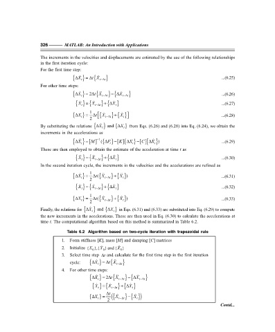
time t. The computational algorithm based on this method is summarized in Table 6.2.
Table 6.2 Algorithm based on two-cycle iteration with trapezoidal rule
1. Form stiffness [K], mass [M] and damping [C] matrices

2. Initialize {X 0 },{X 0 } and {X 0 }
3. Select time step t∆ and calculate for the first time step in the first iteration

cycle: {∆ t } = ∆X { t X t− ∆t }
4. For other time steps:

−
2
{∆X t } =∆ { t X t− ∆ } {∆X t− ∆t t }

+
=
X
{ } { X t− ∆t } {∆X t }
t
∆t } { })
{∆X } = { ( X − X
t
2 t− ∆t t
Contd...