Page 59 - MATLAB an introduction with applications

44 ——— MATLAB: An Introduction with Applications

1.20.1 Finding Zeros and Poles of B(s)/A(s)
The MATLAB command [z, p, k] = tf 2zp(num, den) is used to find the zeros (z), poles (p), and gain (k) of
B(s)/A(s).
If the zeros (z), poles (p) and gain (k) are given, the following MATLAB command can be used to find the
original num/den:
[num, den] = zp2tf (z,p,k)

1.21 CONTROL SYSTEMS

MATLAB has an extensive set of functions for the analysis and design of control systems. They involve
matrix operati7ons, root determination, model conversions and plotting of complex functions. These functions
are found in MATLAB’s control systems toolbox. The analytical techniques used by MATLAB for the
analysis and design of control systems assume the processes that are linear and time invariant. MATLAB
uses models in the form of transfer-functions or state-space equations.

1.21.1 Transfer Functions
The transfer function of a linear time invariant system is expressed as a ratio of two polynomials. The transfer
function for a single input and a single output (SISO) system is written as
+
bs n + b s n 1 − + ...+ b s b
H(s) = 0 1 n 1 − n
as m + a s m 1 − + ...+ a m 1 − s + a m
1
0
when the numerator and denominator of a transfer function are factored into the zero-pole-gain form, it is
given by
(s − z )(s − z )...(s − z )
H(s) = k 1 2 n
(s − p 1 )(s − p 2 )...(s − p m )
The state-space model representation of a linear control system s is written as
x = Ax + Bu
y = Cx + Du

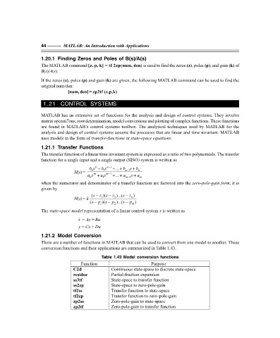
1.21.2 Model Conversion
There are a number of functions in MATLAB that can be used to convert from one model to another. These
conversion functions and their applications are summarized in Table 1.43.

Table 1.43 Model conversion functions
Function Purpose
C2d Continuous state-space to discrete state-space
residue Partial-fraction expansion
ss3tf State-space to transfer function
ss2zp State-space to zero-pole-gain
tf2ss Transfer function to state-space
tf2zp Transfer function to zero-pole-gain
zp2ss Zero-pole-gain to state-space
zp2tf Zero-pole-gain to transfer function

F:\Final Book\Sanjay\IIIrd Printout\Dt. 10-03-09