Page 64 - MATLAB an introduction with applications

MATLAB Basics ——— 49

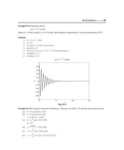
Example E1.9: Generate a plot of
y(x) = e –0.6x cos ωx
where ω = 10 rad/s, and 0 ≤ x ≤ 15. Use the colon notation to generate the x vector in increments of 0.05.

Solution:
>> x=[0:0.1:15];
>> w=10;
>> y=exp(–0.6*x)*cos(w*x);
>> plot(x,y)
>> title(‘y(x)=e^–^0^.^6^xcos\omega x’)
>> xlabel(‘x’)
>> ylabel(‘y’)
ω
() =
yx e − 0.6x cos x
1
0.8
0.6
0.4
0.2

y 0
–0.2
–0.4

–0.6
–0.8
–1
0 5 10 15
x
Fig. E1.9
Example E1.10: Using the functions for plotting x-y data given in Table 1.29, plot the following functions:
2
(a) r = 5 cos 3t; 0 ≤ t ≤ 2π
(b) r = 5 cos 3t; 0 ≤ t ≤ 2π
2
x = r cos t, y = r sin t
(c) y = e –2x cos x; 0 ≤ t ≤ 20
1
y = e 2x
2
cos( )
x
(d) y = ; –5 ≤ x ≤ 5π
x
(e) f = e –3t/5 cos t; 0 ≤ t ≤ 2π
1
(f ) z = − –x + 2xy + y ; |x| ≤ 7, |y| ≤ 7
2
2
3

F:\Final Book\Sanjay\IIIrd Printout\Dt. 10-03-09