
Page 78 - MATLAB an introduction with applications
P. 78
MATLAB Basics ——— 63
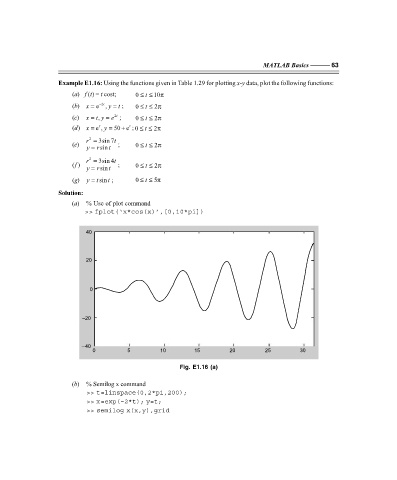
Example E1.16: Using the functions given in Table 1.29 for plotting x-y data, plot the following functions:
(a) f (t) = t cost; 0 ≤≤ 10π
t
−
2t
(b) x = e, = t ; 0 ≤≤ 2π
t
y
2t
(c) x = t , = e ; 0 ≤≤ 2π
y
t
t
t
+
y
(d) x = e, = 50 e ; 0 ≤≤t 2π
r = 3sin 7t
2
(e) y = r sint ; 0 ≤≤ 2π
t
r = 3sin 4t
2
(f ) y = r sin t ; 0 ≤≤ 2π
t
t
(g) y = t sin t ; 0 ≤≤ 5π
Solution:
(a) % Use of plot command
>> fplot(‘x*cos(x)’,[0,10*pi])
40
20
0
–20
–40
0 5 10 15 20 25 30
Fig. E1.16 (a)
(b) % Semilog x command
>> t=linspace(0,2*pi,200);
>> x=exp(–2*t); y=t;
>> semilog x(x,y),grid
F:\Final Book\Sanjay\IIIrd Printout\Dt. 10-03-09