
Page 73 - MATLAB an introduction with applications
P. 73
58 ——— MATLAB: An Introduction with Applications
0.4
0.2
Z 0
–0.2
–0.4
4
2 4
0 2
0
–2 –2
y –4 –4
x
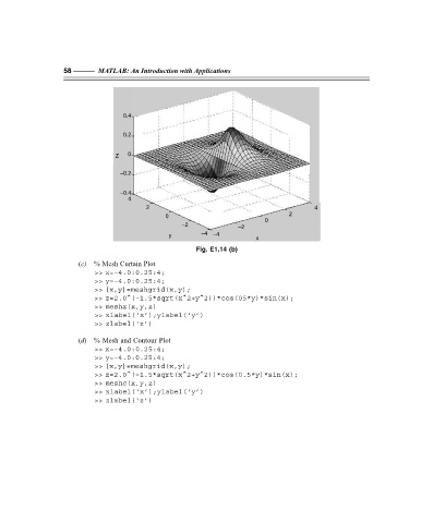
Fig. E1.14 (b)
(c) % Mesh Curtain Plot
>> x=–4.0:0.25:4;
>> y=–4.0:0.25:4;
>> [x,y]=meshgrid(x,y);
>> z=2.0^(–1.5*sqrt(x^2+y^2))*cos(05*y)*sin(x);
>> meshz(x,y,z)
>> xlabel(‘x’);ylabel(‘y’)
>> zlabel(‘z’)
(d) % Mesh and Contour Plot
>> x=–4.0:0.25:4;
>> y=–4.0:0.25:4;
>> [x,y]=meshgrid(x,y);
>> z=2.0^(–1.5*sqrt(x^2+y^2))*cos(0.5*y)*sin(x);
>> meshc(x,y,z)
>> xlabel(‘x’);ylabel(‘y’)
>> zlabel(‘z’)
F:\Final Book\Sanjay\IIIrd Printout\Dt. 10-03-09