
Page 75 - MATLAB an introduction with applications
P. 75
60 ——— MATLAB: An Introduction with Applications
0.5
0
–0.5
5
5
0
0
y –5 –5 x
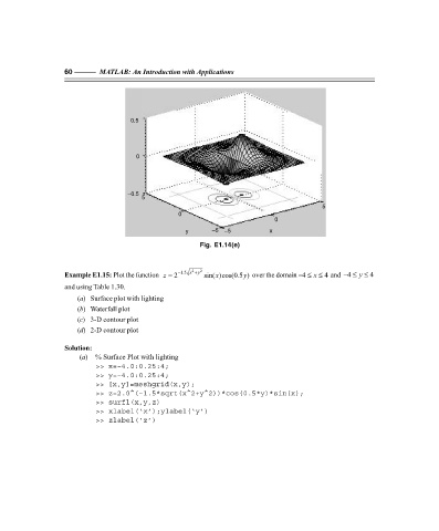
Fig. E1.14(e)
−≤ y
Example E1.15: Plot the function = 2 − 1.5 x 2 +y 2 sin( )cos(0.5 ) over the domain 4−≤ x ≤ 4 and 4 ≤ 4
y
z
x
and using Table 1.30.
(a) Surface plot with lighting
(b) Waterfall plot
(c) 3-D contour plot
(d) 2-D contour plot
Solution:
(a) % Surface Plot with lighting
>> x=–4.0:0.25:4;
>> y=–4.0:0.25:4;
>> [x,y]=meshgrid(x,y);
>> z=2.0^(–1.5*sqrt(x^2+y^2))*cos(0.5*y)*sin(x);
>> surfl(x,y,z)
>> xlabel(‘x’);ylabel(‘y’)
>> zlabel(‘z’)
F:\Final Book\Sanjay\IIIrd Printout\Dt. 10-03-09