Page 132 - MATLAB Recipes for Earth Sciences

126 6 Signal Processing

output y(t ). We can easily illustrate this by generating a random signal
n
clear
t = (1:100)';
randn('seed',0);
x1 = randn(100,1);

designing a filter that averages three data points of the input signal

b1 = [1 1 1]/3;
and convolving the input vector with the fi lter

y1 = conv(b1,x1);
The elements of b1 are the weights of the filter. In our example, all fi lter

weights are the same and they equal 1/3. Note that the conv function yields
a vector that has the length n+m-1, where m is the length of the fi lter.

m1 = length(b1);
We should explore the contents of our workspace to check for the length of
the input and output of conv. Typing
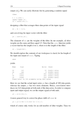
whos

yields

Name Size Bytes Class
b1 1x3 24 double array
m1 1x1 8 double array
t 100x1 800 double array
x1 100x1 800 double array
y1 102x1 816 double array
Grand total is 306 elements using 2448 bytes

Here we see that the actual input series x1 has a length of 100 data points,
whereas the output y1 has two more elements. Hence, convolution intro-
duces (m-1)/2 data points at both ends of the data series. In order to compare
input and output signal, we cut the output signal at both ends.
y1 = y1(2:101,1);

A more general way to correct the phase shifts of conv is

y1 = y1(1+(m1-1)/2:end-(m1-1)/2,1);

which of course only works for an odd number of filter weights. Then we