Page 134 - MATLAB Recipes for Earth Sciences

128 6 Signal Processing

Although the function filter yields an output vector with the same length
as the input vector, we have to correct the output as well. In this case, the
function filter assumes that the fi lter is causal. The fi lter weights are in-
dexed n, n-1, n-2 and so on. Hence, no future elements of the input vector,
such as x(n+1), x(n+2) and so forth are needed to compute the output y(n).

This is of great importance in the field of electrical engineering, the classic

field of application of MATLAB, where filters are often applied in real time.
In earth sciences, however, in most applications the entire signal is available
at the time of processing the data. Filtering the data series is computed by
y4 = filter(b3,1,x3);

and afterwards the phase correction is carried out using
y4 = y4(1+(m3-1)/2:end-(m3-1)/2,1);
y4(end+1:end+m3-1,1)=zeros(m3-1,1);

which only works for an odd number of filter weights. This command sim-

ply shifts the output by(m-1)/3 towards the lower end of the t-axis, then

fills the end of the data series by zeros. Comparing the ends of both outputs
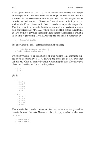
illustrates the effect of this correction, where

y3(1:5,1)
y4(1:5,1)

yields
ans =
0.3734
0.4437
0.3044
0.4106
0.2971

ans =
0.3734
0.4437
0.3044
0.4106
0.2971
This was the lower end of the output. We see that both vectors y3 and y4
contain the same elements. Now we explorer the upper end of the data vec-
tor, where

y3(end-5:end,1)
y4(end-5:end,1)