Page 135 - MATLAB Recipes for Earth Sciences

6.6 Recursive and Nonrecursive Filters 129

causes the output

ans =
0.2268
0.1592
0.3292
0.2110
0.3683
0.2414
ans =
0.2268
0.1592
0
0
0
0

The vectors are identical up to element y(end-m3+1), then the second vec-
tor y4 contains zeros instead of true data values. Plotting the results with

subplot(2,1,1), plot(t,x3,'b-',t,y3,'g-')
subplot(2,1,2), plot(t,x3,'b-',t,y4,'g-')

or in one single plot,

plot(t,x3,'b-',t,y3,'g-',t,y4,'r-')
shows that the results of conv and filter are identical except for the upper
end of the data vector. These observations are important for our next steps in
signal processing, in particular if we are interested in leads and lags between
various components of signals.

6.6 Recursive and Nonrecursive Filters

Now we expand our nonrecursive filters by a recursive component, i.e., the

output y(t ) depends on the fi lter input x(t), but also on previous output val-
n
ues y(t ), y(t ), y(t ). This fi lter requires the nonrecursive fi lter weights b ,
n-1 n-2 n-3 i
but also the recursive fi lters weights a (Fig. 6.2). This fi lter can be described
i
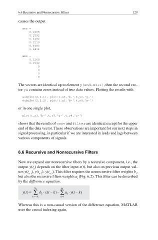
by the difference equation.

Whereas this is a non-causal version of the difference equation, MATLAB
uses the causal indexing again,