Page 133 - MATLAB Recipes for Earth Sciences

6.5 Comparing Functions for Filtering Data Series 127

can plot both input and output signals for comparison. We also use legend
to display a legend for the plot.

plot(t,x1,'b-',t,y1,'r-')
legend('x1(t)','y1(t)')

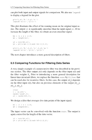
This plot illustrates the effect of the running mean on the original input se-
ries. The output y1 is signifi cantly smoother than the input signal x1. If we

increase the length of the filter, we obtain an even smoother signal.
b2 = [1 1 1 1 1]/5;
m2 = length(b2);

y2 = conv(b2,x1);
y2 = y2(1+(m2-1)/2:end-(m2-1)/2,1);
plot(t,x1,'b-',t,y1,'r-',t,y2,'g-')
legend('x1(t)','y1(t)','y2(t)')
The next chapter introduces a more general description of fi lters.

6.5 Comparing Functions for Filtering Data Series

A very simple example of a nonrecursive filter was described in the previ-

ous section. The fi lter output y(t) only depends on the fi lter input x(t) and
the fi lter weights b . Prior to introducing a more general description for
k
linear time-invariant fi lters, we replace the function conv by filter that
can be used also for recursive filters. In this case, the output y(t ) depends

n
on the fi lter input x(t), but also on previous elements of the output y(t ),
n-1
y(t ), y(t ).
n-2 n-3
clear
t = (1:100)';
randn('seed',0);
x3 = randn(100,1);

We design a filter that averages five data points of the input signal.
b3 = [1 1 1 1 1]/5;
m3 = length(b3);

The input vector can be convolved with the function conv. The output is
again correct for the length of the data vector.

y3 = conv(b3,x3);
y3 = y3(1+(m3-1)/2:end-(m3-1)/2,1);