Page 138 - MATLAB Recipes for Earth Sciences

132 6 Signal Processing

Unit Impulse Impulse Response
2 2

1 1

y(t) 0 y(t) 0

ï1 ï1

ï2 ï2
0 5 10 15 20 0 5 10 15 20
t t
a b
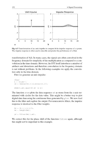
Fig. 6.3 Transformation of a a unit impulse to compute b the impulse response of a system.
The impulse response is often used to describe and predict the performance of a fi lter.

transformation of Y(f). In many cases, the signals are often convolved in the
frequency domain for simplicity of the multiplication as compared to a con-
volution in the time domain. However, the FFT itself introduces a number of
artifacts and distortions and therefore convolution in the frequency domain
is not without problems. In the following examples we apply the convolu-
tion only in the time domain.
First we generate an unit impulse:

clear
t = (0:20)';
x6 = [zeros(10,1);1;zeros(10,1)];

stem(t,x6),axis([0 20 -4 4])
The function stem plots the data sequence x6 as stems from the x-axis ter-
minated with circles for the data value. This might be a better way to plot
digital data than using the continuous lines generated by plot. We now feed
this to the filter and explore the output. For nonrecursive filters, the impulse

response is identical to the fi lter weights.
b6 = [1 1 1 1 1]/5;
m6 = length(b6);
y6 = filter(b6,1,x6);

We correct this for the phase shift of the function filter again, although
this might not be important in this example.