Page 189 - MATLAB Recipes for Earth Sciences

184 7 Spatial Data

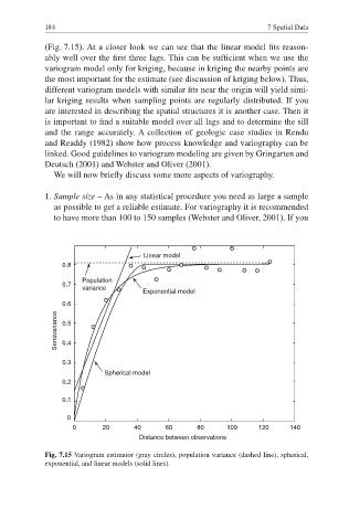
(Fig. 7.15). At a closer look we can see that the linear model fi ts reason-

ably well over the first three lags. This can be sufficient when we use the
variogram model only for kriging, because in kriging the nearby points are
the most important for the estimate (see discussion of kriging below). Thus,
different variogram models with similar fi ts near the origin will yield simi-
lar kriging results when sampling points are regularly distributed. If you
are interested in describing the spatial structures it is another case. Then it

is important to find a suitable model over all lags and to determine the sill
and the range accurately. A collection of geologic case studies in Rendu
and Readdy (1982) show how process knowledge and variography can be
linked. Good guidelines to variogram modeling are given by Gringarten and
Deutsch (2001) and Webster and Oliver (2001).

We will now briefly discuss some more aspects of variography.
1. Sample size – As in any statistical procedure you need as large a sample
as possible to get a reliable estimate. For variography it is recommended
to have more than 100 to 150 samples (Webster and Oliver, 2001). If you

Linear model
0.8

Population
0.7
variance
Exponential model
0.6
Semivariance 0.5

0.4
0.3
Spherical model
0.2
0.1

0
0 20 40 60 80 100 120 140
Distance between observations

Fig. 7.15 Variogram estimator (gray circles), population variance (dashed line), spherical,
exponential, and linear models (solid lines).