Page 188 - MATLAB Recipes for Earth Sciences

7.9 Geostatistics (by R. Gebbers) 183

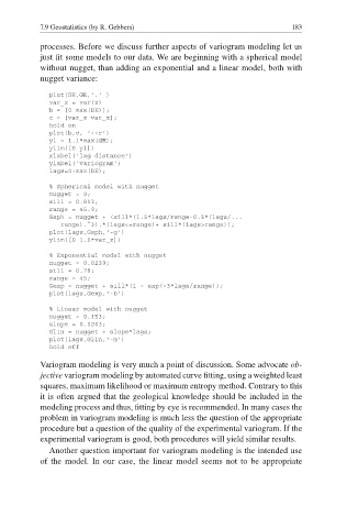
processes. Before we discuss further aspects of variogram modeling let us

just fit some models to our data. We are beginning with a spherical model
without nugget, than adding an exponential and a linear model, both with
nugget variance:

plot(DE,GE,'.' )
var_z = var(z)
b = [0 max(DE)];
c = [var_z var_z];
hold on
plot(b,c, '--r')
yl = 1.1*max(GE);
ylim([0 yl])
xlabel('lag distance')
ylabel('variogram')
lags=0:max(DE);
% Spherical model with nugget
nugget = 0;
sill = 0.803;
range = 45.9;
Gsph = nugget + (sill*(1.5*lags/range-0.5*(lags/...
range).^3).*(lags<=range)+ sill*(lags>range));
plot(lags,Gsph,'-g')
ylim([0 1.1*var_z])
% Exponential model with nugget
nugget = 0.0239;
sill = 0.78;
range = 45;
Gexp = nugget + sill*(1 - exp(-3*lags/range));
plot(lags,Gexp,'-b')
% Linear model with nugget
nugget = 0.153;
slope = 0.0203;
Glin = nugget + slope*lags;
plot(lags,Glin,'-m')
hold off

Variogram modeling is very much a point of discussion. Some advocate ob-

jective variogram modeling by automated curve fitting, using a weighted least
squares, maximum likelihood or maximum entropy method. Contrary to this
it is often argued that the geological knowledge should be included in the
modeling process and thus, fitting by eye is recommended. In many cases the

problem in variogram modeling is much less the question of the appropriate
procedure but a question of the quality of the experimental variogram. If the
experimental variogram is good, both procedures will yield similar results.
Another question important for variogram modeling is the intended use
of the model. In our case, the linear model seems not to be appropriate