Page 183 - MATLAB Recipes for Earth Sciences

178 7 Spatial Data

where srqt is the square root of the data. Then we get the experimental
variogram G as half the squared differences between the observed values:

G = 0.5*(Z1 - Z2).^2;

We used the MATLAB capability to vectorize commands instead of us-
2
ing for loops in order to run faster. However, we have computed n pairs
of observations although only n*(n-1)/2 pairs are required. For large data
sets, e.g., more than 3000 data points, the software and physical memory
of the computer may become a limiting factor. For such cases, a more ef-

ficient way of programming is described in the user manual of the software
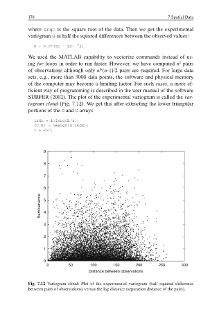
SURFER (2002). The plot of the experimental variogram is called the var-
iogram cloud (Fig. 7.12). We get this after extracting the lower triangular
portions of the D and G arrays

indx = 1:length(z);
[C,R] = meshgrid(indx);
I = R>C;

9

8

7

6
Semivariance 5 4

3

2

1

0
0 50 100 150 200 250 300
Distance between observations

Fig. 7.12 Variogram cloud: Plot of the experimental variogram (half squared difference
between pairs of observations) versus the lag distance (separation distance of the pairs).