Page 181 - MATLAB Recipes for Earth Sciences

176 7 Spatial Data

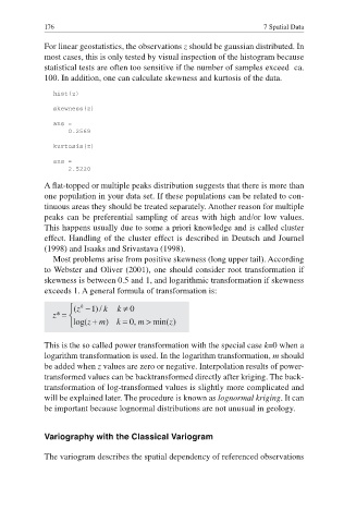
For linear geostatistics, the observations z should be gaussian distributed. In
most cases, this is only tested by visual inspection of the histogram because
statistical tests are often too sensitive if the number of samples exceed ca.
100. In addition, one can calculate skewness and kurtosis of the data.
hist(z)

skewness(z)
ans =
0.2568

kurtosis(z)
ans =
2.5220

Aflat-topped or multiple peaks distribution suggests that there is more than

one population in your data set. If these populations can be related to con-
tinuous areas they should be treated separately. Another reason for multiple
peaks can be preferential sampling of areas with high and/or low values.
This happens usually due to some a priori knowledge and is called cluster
effect. Handling of the cluster effect is described in Deutsch and Journel
(1998) and Isaaks and Srivastava (1998).
Most problems arise from positive skewness (long upper tail). According
to Webster and Oliver (2001), one should consider root transformation if
skewness is between 0.5 and 1, and logarithmic transformation if skewness
exceeds 1. A general formula of transformation is:

This is the so called power transformation with the special case k=0 when a
logarithm transformation is used. In the logarithm transformation, m should
be added when z values are zero or negative. Interpolation results of power-
transformed values can be backtransformed directly after kriging. The back-
transformation of log-transformed values is slightly more complicated and
will be explained later. The procedure is known as lognormal kriging. It can
be important because lognormal distributions are not unusual in geology.

Variography with the Classical Variogram

The variogram describes the spatial dependency of referenced observations