Page 176 - MATLAB Recipes for Earth Sciences

7.8 Comparison of Methods and Potential Artifacts 171

120 20
20 5 5
15
115 0 15
–15
–10 –15
20 15 –10
110 20 20 –20 10
–5 5
20 –25 –10 5
–15
105 15 5 –20
–5
–25
–25
15 0
100 15 –15
–20
15 –10 –20 –10 0 −5
–20
95 –20 –5
–5 –15
–10
10 10 10 –10 –10–15–15 −10
–10
–10
–10
90 –15
−15
10 –5 0
85 10 –10 –5
–20 –15 −20
–10
–20 5
80 –20 –15 –5
–15
15 –15 –10 0 −25
–15
–15
75 0 −30
15 5 0 5
15 5
70 −35
420 425 430 435 440 445 450 455 460 465 470
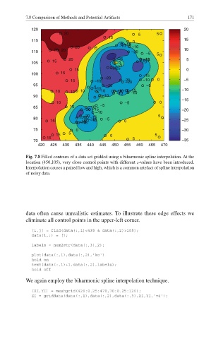
Fig. 7.8 Filled contours of a data set gridded using a biharmonic spline interpolation. At the
location (450,105), very close control points with different z-values have been introduced.
Interpolation causes a paired low and high, which is a common artefact of spline interpolation
of noisy data.
data often cause unrealistic estimates. To illustrate these edge effects we
eliminate all control points in the upper-left corner.
[i,j] = find(data(:,1)<435 & data(:,2)>105);
data(i,:) = [];
labels = num2str(data(:,3),2);
plot(data(:,1),data(:,2),'ko')
hold on
text(data(:,1)+1,data(:,2),labels);
hold off
We again employ the biharmonic spline interpolation technique.

[XI,YI] = meshgrid(420:0.25:470,70:0.25:120);
ZI = griddata(data(:,1),data(:,2),data(:,3),XI,YI,'v4');