Page 175 - MATLAB Recipes for Earth Sciences

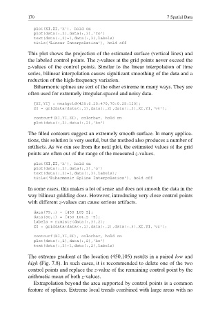
170 7 Spatial Data

plot(XI,ZI,'k'), hold on
plot(data(:,1),data(:,3),'ro')
text(data(:,1)+1,data(:,3),labels)
title('Linear Interpolation'), hold off

This plot shows the projection of the estimated surface (vertical lines) and
the labeled control points. The z-values at the grid points never exceed the
z-values of the control points. Similar to the linear interpolation of time

series, bilinear interpolation causes significant smoothing of the data and a
reduction of the high-frequency variation.
Biharmonic splines are sort of the other extreme in many ways. They are
often used for extremely irregular-spaced and noisy data.

[XI,YI] = meshgrid(420:0.25:470,70:0.25:120);
ZI = griddata(data(:,1),data(:,2),data(:,3),XI,YI,'v4');
contourf(XI,YI,ZI), colorbar, hold on
plot(data(:,1),data(:,2),'ko')

The fi lled contours suggest an extremely smooth surface. In many applica-
tions, this solution is very useful, but the method also produces a number of
artifacts. As we can see from the next plot, the estimated values at the grid
points are often out of the range of the measured z-values.

plot(XI,ZI,'k'), hold on
plot(data(:,1),data(:,3),'o')
text(data(:,1)+1,data(:,3),labels);
title('Biharmonic Spline Interpolation'), hold off

In some cases, this makes a lot of sense and does not smooth the data in the
way bilinear gridding does. However, introducing very close control points
with different z-values can cause serious artifacts.

data(79,:) = [450 105 5];
data(80,:) = [450 104.5 -5];
labels = num2str(data(:,3),2);
ZI = griddata(data(:,1),data(:,2),data(:,3),XI,YI,'v4');
contourf(XI,YI,ZI), colorbar, hold on
plot(data(:,1),data(:,2),'ko')
text(data(:,1)+1,data(:,2),labels)

The extreme gradient at the location (450,105) results in a paired low and
high (Fig. 7.8). In such cases, it is recommended to delete one of the two
control points and replace the z-value of the remaining control point by the
arithmetic mean of both z-values.
Extrapolation beyond the area supported by control points is a common
feature of splines. Extreme local trends combined with large areas with no